All published articles of this journal are available on ScienceDirect.

Parameter Prioritization in Techno-economic Model for Decision-making in the Petrochemicals Industry
Abstract
Introduction/Objective
The petrochemical industry plays a pivotal role in the global economy but continues to face significant challenges, including fluctuating oil prices, tightening environmental regulations, and high capital investment requirements. Hence, reliable techno-economic models are essential when companies approach Final Investment Decisions (FID), which determine the success of large-scale projects.
Method
This study introduces a structured framework that prioritises and ranks the parameters that are most critical to such models. The approach combines the Objective Weighting Method (OWM) with the Technique for Order Preference by Similarity to Ideal Solution (TOPSIS) by using propylene oxide production as a case study.
Results
The analysis discloses that the total revenue is the highest-priority parameter (Pi = 0.5280), followed by raw material cost (0.4576), utilities cost (0.2316), investment cost (0.2209), and fixed cost (0.1905).
Discussion
By identifying the most influential parameters, this approach enables decision-makers to allocate resources more effectively, improve cost efficiency, and reduce uncertainty. When combined with sensitivity analysis, it empowers companies to assess the impact of changing conditions, thus strengthening risk management and increasing the likelihood of project success in an uncertain and highly competitive sector.
Conclusion
The Structured Entropy-TOPSIS framework is a strong, evidence-based tool that identifies the key factors in petrochemical investment decisions. The findings decrease decision-making uncertainty while increasing the chances of the project being successful, as management attention is directed towards the economic variables with high impact.
1. INTRODUCTION
The Final Investment Decision (FID) is a crucial milestone in the advancement of large-scale petrochemical projects [1]. It signifies the point at which project owners grant approval for the project's continued advancement and inform investors and the public that they have secured the required money and anticipate future financial gains [2]. The board of directors usually finalizes the FID after accomplishing many critical project development milestones, including feasibility studies, pre-FEED, FEED, and EPC phases [3]. The FID decision is an intricate procedure that entails assessing a variety of techno-economic aspects. These characteristics are crucial in assessing the project's feasibility and likelihood of achieving success [4]. During the FID process, the techno-economic parameters must be systematically prioritized to account for their varying impact on the project [5].
The FID process takes into account various factors, including total investment costs, product spread, taxes, weighted average cost of capital, and operational costs. Technical characteristics, such as the availability of resources, the timeline of the project, and the impact on the environment, are important factors that influence the FID decision [2]. For instance, project feasibilities are influenced by the availability of raw materials and workforce. Another factor that may directly influence the final project costs is the project schedule, as any delays will result in additional expenses. Environmental impact also plays a critical role, particularly in situations where projects may face delays due to approval or mitigation requirements.
Commanding an informed decision on final investments depends on prioritizing and ranking those techno-economics parameters. The establishment of a thorough feasibility study, for instance, by comparing the cost of buying utilities versus building them, helps determine the economic viability of the project [6]. Through the feasibility study, the project’s financial returns, technical viability, and environmental impacts can be better understood [2]. The analysis also highlights potential risks and uncertainties associated with the project, including cost overruns or schedule delays caused by procurement issues. A step forward after the study completion is the development of a detail project plan which includes specific timelines and budget estimates. The plan defines the scope of activities, key milestones, and the overall flow of actions, including mobilization, construction, commissioning, and initial acceptance. Potential hazards and mitigation measures were also identified to minimize their impact, for instance, addressing safety risks during heavy lifting or working at height. It is a strategic guide that assists the project in staying on track and ensuring it continues to meet the objectives. One of the key steps in the FID process is conducting a proper assessment of potential risks and providing measures to reduce them [7]. Early identification of risks, such as raw material price fluctuations or delays caused by contractor availability, allows the project owner to plan appropriate mitigation actions. These may include contingency plans, insurance coverage, and arrangements for risk sharing. Project owners can reduce uncertainty and improve the likelihood of achieving project targets.
The FID process also evaluates different sensitivities and scenarios [8], such as the robustness of the project under varying market pressure or challenging operating conditions. For instance, project economics will be examined by assessing base, best, and worst-case demand scenarios to understand the impact. Sensitivity analysis, on the other hand, permits companies to assess the project's response to market demand, feedstock prices, and changes in total investment cost and operating expenses. With the intention of attaining the FID decision, companies often use anticipated value analysis, Monte Carlo simulation, and multi-criteria decision-making [9]. These tools provide a systematic approach to the evaluation of the future expected payback of the project and risk profile. They enable the owners of a project to make informed decisions that are keen on considering technical, economic, and environmental issues.
Finally, the FID decision is an essential milestone in the development of large-scale petrochemical projects. A thorough assessment of techno-economic factors is for a well-informed choice. This is because the owners of the projects can balance technical, economic, and environmental factors by allocating the priority and ranking of these aspects and thus increasing the chances of success [6]. These techno-economic parameters must be prioritized and ranked to make an informed FID decision, to have the project suit the necessary requirements for investments. This may involve undertaking comprehensive feasibility studies to determine the economic viability of the project, devising an elaborate project plan with timelines and budget estimates, identifying and eliminating project risks, assessing alternative scenarios and sensitivities in order to ensure strength, and also application of expected value analysis, Monte Carlo simulation, and multi-criteria decision-making analysis, which will estimate the probability of success. Companies can make informed investment decisions by prioritizing and ranking techno-economic parameters that balance technical, economic, and environmental considerations [5]. This approach can help mitigate risks and increase the chances of project success.
2. LITERATURE REVIEW
2.1. Background of the Malaysian Economy and the Petrochemicals Industry
Malaysia's ethylene market is dominated by High-Density Polyethylene (HDPE), Low-Density Polyethylene (LDPE), and Ethylene Oxide (EO). Since Vinyl Chloride Malaysia (a PETRONAS subsidiary) exited the vinyl business in late 2012, there has been no more ethylene demand for EDC and VCM. The recent drop in ethylene demand is also due to HDPE losing its market competitiveness. Although local demand for HDPE continues to grow, limited production capacity has resulted in increased imports from the Middle East to meet the demand gap. Currently, downstream production will increase as a result of a more competitive ethylene supply from the expanded cracker, followed by a 70% increase from the Pengerang Integrated Complex (PIC). The complex will have the potential to generate one million tonnes of ethylene per year and will also have HDPE and Linear Low-Density Polyethylene (LLDPE) production capabilities [10]. In Malaysia, PETRONAS Chemical Ethylene Malaysia, Lotte Chemical Titan, and PETRONAS Chemical Olefins Malaysia operate ethylene crackers. Lotte Chemical Titan, located in Pasir Gudang, is the largest manufacturer, with a combined capacity of 735,000 metric tonnes per year. Lotte Chemical Titan expanded its ethylene capacity by 90,000 tonnes per year in August 2017, after Malaysia's ethylene capacity had been stable for a long time. This expansion utilized catalytic cracking, which was combined with the existing naphtha thermal cracker to create the world's first hybrid ethylene-producing facility. The massive new PETRONAS refinery and naphtha-based steam cracker project with a design capacity of 1.3 million metric tonnes per annum of ethylene is more substantial than the polyethylene, polypropylene, and Mono Ethylene Glycol projects (MEG) [10].
Polypropylene accounted for over 55% of Malaysia's propylene demand, with oxo-alcohols and acrylic acid also being significant consumers. Since 2008, Malaysia's annual propylene capacity has been slightly over one million metric tonnes. Nonetheless, the market for propylene in Malaysia will experience substantial shifts during the forecast period. In August of 2017, Lotte Chemical Titan expanded its naphtha cracker, increasing annual propylene capacity by 160,000 metric tonnes, while the steam cracker in Pengerang will produce roughly 660,000 metric tonnes of propylene and polypropylene per year [11]. The first butadiene rubber plant in Malaysia was inaugurated at the end of 2015, with an annual capacity of 50,000 tonnes of butadiene, or roughly a quarter of historical usage levels [12]. In recent years, the rise of NBR latex production has been the key demand driver for butadiene in Malaysia. Malaysia is the world's leading provider of natural rubber and NBR gloves, with a 60% market share. In recent years, the demand for NBR gloves has steadily outpaced that for natural rubber gloves [13]. Butadiene consumption in NBR latex will continue to fuel expansion, as rising health care expenditures, ageing populations, and higher global cleanliness standards will increase the need for medical gloves [14]. By the third quarter of 2018, Synthomer increased its capacity by 90,000 tonnes per year, bringing the total to 270,000 tonnes per year [15]. This expansion will push local demand for butadiene up to 30,000 tonnes. Another contributor is Toray Plastics; their recent expansion means ABS is now a small but growing part of butadiene usage here. Earlier in March 2008, Titan Petrochemicals started its 100,000 tonne per year butadiene plant, before the whole company was bought by Honam Corporation from South Korea. This plant uses “mixed C4” from its own steam cracker, which used to be exported. Currently, about 50% of the butadiene produced is sent to Kumho Petrochemical in South Korea. In 2020, PETRONAS began supplying 1.3 million tonnes of feed yearly to the RAPID naphtha-based steam cracker. This complex includes a distillation plant that can produce 190,000 tonnes of butadiene every year [16].
Many factors have affected the performance, profit, and investment levels of the global petrochemical industry. This includes environmental rules, new technology, changes in what customers want, and global politics or economic issues.
For Malaysia, one of the biggest challenges is the shortage of resources. It is very important that our offshore fields can still supply oil and gas feedstock at a lower price compared to other countries. This low cost is what allows Malaysia to produce petrochemical products at a competitive price. To stay ahead, Malaysia must make sure these prices remain low. In terms of total capacity, Malaysia’s crude oil reserves rank 28th in the world (573,000 barrels per day), while our natural gas reserves rank 12th (74.2 billion cubic meters) [17]. Malaysia also boasts the world's largest LNG production facility, with an annual output of 29.3 million metric tons, located on its territory [16]. Despite having such a large oil reserve, Malaysia is actually a net importer of the commodity due to falling domestic production in recent decades. Malaysia also has some of the world's most advanced oil refineries, with a combined daily output of 955 thousand barrels from its five operational refineries [17].
The petrochemical industries must use robust technology to optimize the available resources. Companies should also keep looking for new technology and inventive applications for the ones they currently have. If the petrochemical sector does not evolve in this manner, it will fall behind the market and lose any advantages it may have. The necessity for qualified labor capable of handling the complexities of the petrochemical business should also be considered. Nevertheless, basic training may not be enough to provide the company with a competitive advantage over competitors who may have more qualified employees. Lastly, the environment is severely impacted as a result of carbon dioxide overproduction, and the petrochemical industry is responsible for the majority of these emissions. It will be critical for industry players to solve it by redesigning new and existing operations to produce less carbon dioxide [18].
2.2. Background of Selected Petrochemicals Production
Propylene oxide is a component in the synthesis of polyether polyols, propylene glycols, and other specialized chemicals. In the 1970s, Chlorohydrin (CHPO) or chlorohydrin with chlor-alkali (CHPO CA) was at the height of its popularity. Essentially, this technique has not been widely adopted in most industrialized nations because of the environmental concerns around chlorine byproducts. The chlorohydrin process still accounts for over 40% of global capacity as of 2016, despite its declining popularity and multiple closures [19]. Other technologies that have been developed by the researchers as substitutes for the chlorohydrin process include Propylene Oxide-Styrene Monomer (POSM) and Propylene Oxide-Tertiary Butyl Alcohol (POTBA) processes. The POSM process started in 1974 because it was a cheaper way to make propylene oxide. Today, it is the second-most used method in the world. Later in 2003, Sumitomo Chemical came out with a new process using cumene hydroperoxide (CuPO). This method is advantageous because it does not produce any extra co-products.
Other companies like Evonik, Dow, and BASF also found a way to make propylene oxide using hydrogen peroxide (the HPPO process). These companies started looking at each other’s work in 2002 and began working together the year after. They eventually built a full-scale HPPO plant at the BASF site in Antwerp, Belgium [19].
2.3. Objective Weighing Method
Objective weighing method is a versatile and effective tool for decision-making, data analysis, and information theory [9, 20]. One of the primary advantages of this method is its ability to provide an objective way to assign weights to different criteria or features based on their variability or uncertainty. This will aid in minimizing the bias during the weighting process, and the weights will not be based on individual opinions or random decisions. The other important advantage of the objective weighing technique is that it deals with uncertainty. This method can be used to provide a more suitable distribution in situations of high uncertainty, as the level of uncertainty or randomness in the data is quantified and more importance is placed on reliable and consistent criteria in the final decision [20].
The most attractive feature of this approach is the data-driven approach. Entropy weighting involves the computation of weights based on the data, as opposed to subjective weighting schemes, which make use of a subjective assessment or arbitrary decisions. This finds it especially applicable in situations when the expert knowledge is incomplete or absent. It is also natural in the ability of the method to normalize data, that is, the weights add to one. This fact simplifies the interpretation and comparison of the results. Moreover, the objective weighing technique is very adaptable, and it may be used in any range of subjects like economics, engineering, environmental science, and multi-criteria decision-making [21].
Moreover, this technique can be utilized to improve decision-making by considering the variability of the data [22]. This leads to more reliable and trustworthy outcomes while facilitating the balancing of different factors, ensuring that no single issue or factor can rule the decision-making process. This can be implemented because the weightages are based on data rather than personal bias. In short, the objective weighing method is a pertinent tool for both researchers and practitioners. The method has the capacity to improve decision-making quality due to its impartiality, ability to handle uncertainty, data-driven nature, and flexible. Consistent and clearer decisions can be made for different projects or technology choices by applying this tool, as it helps manage vagueness and offers comparing options.
2.4. Parameters Prioritization and Rank Parameters Based on Outcome
Prioritizing techno-economic parameters entails examining the most significant factors that influence the performance and viability of a technology or system, and concentrating the analysis on these factors. This ensures that limited resources are concentrated on the most critical issues and that the analysis is concentrated on the most critical information. The second phase of the research entails prioritizing the parameters derived in the first phase, utilizing the MCDM approach. The initial objective of this phase is to evaluate the significance of the parameters prior to prioritization. The MCDM method is regarded as an effective method for aiding decision-making under varying scenarios.
A common MCDM approach is as follows [23]:
Step 1: Identify the type of the problem.
Step 2: Construct a hierarchy of its evaluation.
Step 3: Select the most appropriate model of evaluation.
Step 4: Analyze the relative performance scores and the weights of each attribute relative to each alternative.
Step 5: Pick the best alternative based on the synthetic expected utility, which is the total of relative weights and performance ratings given to the alternatives. When the sum scores of the options are not definite, it will be helpful to insert Step 6 to establish a ranking and thereby make selecting the best alternative straightforward.
Step 6: Compare the alternatives on the basis of the synthetic values derived using fuzzy logic in Step 5.
2.5. Technique for Order Preference by Similarity to Ideal Solution
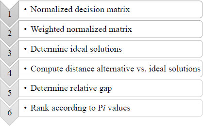
The Technique for Order Preference by Similarity to Ideal Solution is a ranking method that selects the most preferred alternative based on its proximity to the positive ideal solution and its distance from the negative ideal solution simultaneously [24]. A positive ideal solution refers to a solution that maximizes the desirable features and minimizes the undesirable attributes, and vice versa [22]. The TOPSIS technique offers four significant advantages, which are as follows: The logic of TOPSIS is rational and understandable. The calculation methods are straightforward, and the concept enables the identification of the best alternatives for each criterion using a simple mathematical representation. Additionally, the comparison operations incorporate the consideration of importance weights [25]. Regrettably, the TOPSIS technique has a primary drawback in that it incorporates a ranking index that takes into account distances from the ideal and negative-ideal points, but fails to examine their relative importance [26]. However, [27] adhered to the original approach, which includes the six successive steps of the TOPSIS approach operations as outlined by [28] as depicted in Fig. (1).
3. METHODS
3.1. Parameters Prioritization and Ranking
A number of important parameters comprise the total investment cost per tonnage of production, the annual cost of raw materials per tonnage of production, the annual cost of utilities per tonnage of production, the annual fixed cost per tonnage of production, and the total revenue per tonnage of production are collected from six various processes of producing propylene oxide. Prior to solving MCDM problems, it is imperative to determine the weighted average of each technology route comparatively from each other. For the determination of the weighted average, the entropy method was selected because it is purely data-driven. It assigns weights based on the variability and uncertainty within the data itself, reducing the influence of subjective judgments [29]. In this study, the focus is on ranking the techno-economic parameters instead of the technology routes to see which parameter is the most important across the six different ways to produce propylene oxide. For a fair comparison, all parameters were calculated based on one tonne of production.
3.2. Entropy Method to Determine Weighted Average
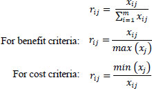
The entropy method is an objective weighting approach widely applied in multi-criteria decision-making, performance evaluation, and composite index construction. It assigns weights to criteria based on their degree of variability (information content) within the dataset. Total Revenue is treated as a benefit criterion, where higher values are preferred. In contrast, Investment Cost, Raw Material Cost, Utilities Cost, and Fixed Cost are treated as cost criteria, where lower values are preferred. The procedure contains three core steps:
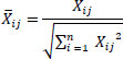
Step 1: Normalized the decision matrix with the help of Eq. (1),
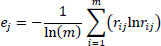
Step 2: Compute the entropy using Eq. (2),
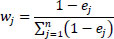
Step 3: Calculate the weight vector using Eq. (3),
3.3. TOPSIS to Prioritize and Rank the Parameters
In this study, the TOPSIS method will be used to evaluate and rank alternatives based on their closeness to an ideal solution. The principle is that the best alternative should have the shortest distance from the Positive Ideal Solution (PIS), representing the most desirable performance, and the farthest distance from the Negative Ideal Solution (NIS), representing the least desirable performance. The procedure involves seven main steps, as follows:
Step 1: Calculate Normalized Matrix using Eq. (4),
Step 2: Calculate the weighted Normalized Matrix using Eq. (5),

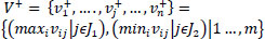
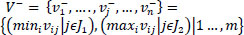
Step 3: Determine positive ideal solution with Eq. (6), negative ideal solutions with Eq. (7),
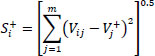
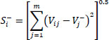
Step 4: Calculate the Euclidean distance from the ideal best using Eq. (8),
Step 5: Calculate the Euclidean distance from the ideal best using Eq. (9),
Step 6: Calculate performance score using Eq. (10),

Step 7: Ranking the performance score
4. RESULTS AND DISCUSSIONS
The case study comparison includes six propylene oxide processes. This section shows the outcome of using parameters and assumptions in OWM and then TOPSIS. Table 1 illustrates the techno-economics parameters value per tonnage of propylene oxide production. Table 2 illustrates normalization of original data from Table 1 and Table 3 shows natural logarithm of the entropy probability matrix, rijlnrij, of data from Table 2. Lastly, Table 4 shows the sums and entropy weights. The detailed entropy weighting calculations are provided in Appendix A.
| Parameters | CHPO CA | CHPO | POSM | POTBA | HPPO | CuPO |
|---|---|---|---|---|---|---|
| Investment Cost | 246 | 102 | 284 | 262 | 226 | 248 |
| Total Revenue | 1745 | 1715 | 4734 | 3606 | 1614 | 1631 |
| Raw Material Cost | 840 | 1763 | 2837 | 2040 | 1060 | 885 |
| Utilities Cost | 188 | 77 | 231 | 135 | 118 | 228 |
| Fixed Cost | 212 | 75 | 246 | 250 | 178 | 214 |
| Parameters | CHPO CA | CHPO | POSM | POTBA | HPPO | CuPO |
|---|---|---|---|---|---|---|
| Investment Cost | 0.4146 | 1.0000 | 0.3592 | 0.3893 | 0.4513 | 0.4113 |
| Total Revenue | 0.3686 | 0.3623 | 1.0000 | 0.7617 | 0.3409 | 0.3445 |
| Raw Material Cost | 1.0000 | 0.4765 | 0.2961 | 0.4118 | 0.7925 | 0.9492 |
| Utilities Cost | 0.4096 | 1.0000 | 0.3333 | 0.5704 | 0.6525 | 0.3377 |
| Fixed Cost | 0.3538 | 1.0000 | 0.3049 | 0.3000 | 0.4213 | 0.3505 |
| Parameters | CHPO CA | CHPO | POSM | POTBA | HPPO | CuPO |
|---|---|---|---|---|---|---|
| Investment Cost | -1.8151 | -1.3451 | -1.8541 | -1.8326 | -1.7734 | -1.7611 |
| Total Revenue | -1.9328 | -2.3605 | -0.8301 | -1.1614 | -2.0539 | -1.9382 |
| Raw Material Cost | -0.9348 | -2.0865 | -2.0472 | -1.7765 | -1.2104 | -0.9248 |
| Utilities Cost | -1.8274 | -1.3451 | -1.9287 | -1.4507 | -1.4047 | -1.9582 |
| Fixed Cost | -1.9739 | -1.3451 | -2.0179 | -2.0932 | -1.8421 | -1.9211 |
| Parameters | CHPO CA | CHPO | POSM | POTBA | HPPO | CuPO |
|---|---|---|---|---|---|---|
| Sum | -1.5105 | -1.5330 | -1.4651 | -1.5556 | -1.5619 | -1.5061 |
| ej | 0.9385 | 0.9524 | 0.9103 | 0.9665 | 0.9704 | 0.9358 |
| dj | 0.0615 | 0.0475 | 0.0897 | 0.0335 | 0.0295 | 0.0642 |
| Wj (%) | 18.87 | 14.58 | 27.52 | 10.27 | 9.06 | 19.70 |
4.1. Prioritization and Ranking Results from the TOPSIS Method
Table 5 indicates the weighted normalized parameter matrix per production, while Table 6 consists of a parameter matrix that has been weighted and normalized for each ton of production. Table 7 contains both positive and negative ideal solutions, while Table 8 indicates performance score results and techno-economic parameter ranking. The detailed TOPSIS calculation for the highest-ranked parameter, Total Revenue, is provided in Appendix B.
| Parameters | CHPO CA | CHPO | POSM | POTBA | HPPO | CuPO |
|---|---|---|---|---|---|---|
| Investment Cost | 0.328 | 0.546 | 0.301 | 0.339 | 0.362 | 0.345 |
| Total Revenue | 0.291 | 0.198 | 0.839 | 0.664 | 0.274 | 0.289 |
| Raw Material Cost | 0.790 | 0.260 | 0.248 | 0.359 | 0.636 | 0.795 |
| Utilities Cost | 0.324 | 0.546 | 0.280 | 0.497 | 0.524 | 0.283 |
| Fixed Cost | 0.280 | 0.546 | 0.256 | 0.261 | 0.338 | 0.294 |
| Parameters | CHPO CA | CHPO | POSM | POTBA | HPPO | CuPO |
|---|---|---|---|---|---|---|
| Investment Cost | 0.0618 | 0.0796 | 0.0829 | 0.0349 | 0.0328 | 0.0679 |
| Total Revenue | 0.0550 | 0.0288 | 0.2309 | 0.0682 | 0.0248 | 0.0568 |
| Raw Material Cost | 0.1492 | 0.0379 | 0.0684 | 0.0369 | 0.0576 | 0.1566 |
| Utilities Cost | 0.0611 | 0.0796 | 0.0770 | 0.0511 | 0.0475 | 0.0557 |
| Fixed Cost | 0.0528 | 0.0796 | 0.0704 | 0.0269 | 0.0306 | 0.0578 |
| CHPO CA | CHPO | POSM | POTBA | HPPO | CuPO | |
|---|---|---|---|---|---|---|
| V+ | 0.1492 | 0.0796 | 0.2309 | 0.0682 | 0.0576 | 0.1566 |
| V- | 0.0528 | 0.0288 | 0.0684 | 0.0269 | 0.0248 | 0.0557 |
| Parameters | Si+ | Si- | Pi | Rank |
|---|---|---|---|---|
| Investment Cost | 0.1978 | 0.0561 | 0.2209 | 4 |
| Total Revenue | 0.1499 | 0.1677 | 0.5280 | 1 |
| Raw Material Cost | 0.1707 | 0.1440 | 0.4576 | 2 |
| Utilities Cost | 0.2050 | 0.0618 | 0.2316 | 3 |
| Fixed Cost | 0.2174 | 0.0512 | 0.1905 | 5 |
4.2. Robustness Analysis Using Monte Carlo Simulation
A Monte Carlo simulation was performed to evaluate the robustness of the Entropy-TOPSIS ranking, which involved all the original input parameters with ±10% variations. This uncertainty range was applied to reflect potential uncertainty in the techno-economic estimates, such as investment cost, total revenue, raw material cost, utilities cost, and fixed cost. The Entropy-TOPSIS procedure was repeated for each iteration of the simulation, and the ranking was compared with that of the base case ranking.
The results indicate that the total revenue and raw material cost remained in the top two parameters in 100% of simulation runs. This corroborates the major conclusion of the study, which is that total revenue and raw materials cost are relatively strong influences on the techno-economic parameters. Utilities cost, and investment cost show some sensitivity in the middle position, indicating that there is some interchangeability under uncertain conditions. Nevertheless, this finding does not impact the key findings of the study (Table 9).
| Parameters | Base Rank | Mean Pi | Rank Retained (%) | Rank 1 Frequency (%) | Top 2 Frequency (%) | Modal Rank |
|---|---|---|---|---|---|---|
| Investment Cost | 4 | 0.2329 | 60.20 | 0.00 | 0.00 | 4 |
| Total Revenue | 1 | 0.5384 | 84.90 | 84.90 | 100.00 | 1 |
| Raw Material Cost | 2 | 0.4543 | 84.90 | 15.10 | 100.00 | 2 |
| Utilities Cost | 3 | 0.2443 | 62.30 | 0.00 | 0.00 | 3 |
| Fixed Cost | 5 | 0.1960 | 94.80 | 0.00 | 0.00 | 5 |
5. DISCUSSIONS
According to the ranking and prioritization analysis, the total revenue generated per ton of output is identified as the most important factor. This indicator is directly linked to the market potential and competitiveness of the product. Higher revenue per ton not only signifies stronger profitability but also demonstrates the capacity of the technology to create added value in the market. Moreover, it helps indicate the project’s potential financial returns and supports stakeholders in assessing profitability over the longer term, for example, by estimating payback periods and cash flow stability. In the second place, the raw materials per ton of production cost are also a key factor in shaping the cost structure. As raw materials cost often makes a large portion of total production cost, any fluctuation in feedstock prices can have a direct and significant impact on the profit margins. Technologies that consume fewer raw materials or allow flexibility in feedstock sourcing tend to be more competitive. The utilities cost per ton of production is considered the third most important factor in evaluating techno-economics performance. Utilities costs per ton reflect the actual consumption of energy and water, providing a clear picture of the ongoing resources needed to keep the facility operating. While this factor is often seen as secondary, it becomes a major factor in high-energy-consumption industries, where sudden spikes in utility prices can blow the entire production cost. For example, a sharp rise in natural gas prices can instantly turn a profitable plant into a loss. While the three main pillars of economic feasibility are imperative, the other cost related factor also play a role in the final evaluation. The total investment cost per ton of production is ranked fourth. This measure reflects the scale of capital required to establish the production facility and provide investors with an early indication of the project's capital intensity. Minimizing the investment cost per ton usually reflects high capital efficiency, making a project stand out in a competitive market where capital is a limited resource. Fixed cost represents the baseline annual expenses that persist regardless of production level, such as staff salaries and administrative overhead. For instance, even during a scheduled maintenance shutdown, these costs remain a constant obligation. Managing them effectively is essential for maintaining financial health in the long term. Overall, the ranking shows that while the upfront investment determines project feasibility at the initial stage, it is the steady revenue and the efficient use of raw materials and utilities that govern the long-term profitability.
6. LIMITATIONS OF THE STUDY
This paper presents an overall prioritization of the techno-economic parameters through the analysis of all major commercial production routes of Propylene oxide that can be found all over the world. Nonetheless, there are some restrictions that should be mentioned to put the findings in context. First, the economic data are (e.g., the prices of raw materials or the utility cost) an instant of the situation on the current market; the major future fluctuations in the global energy or feedstock markets may affect the absolute values of the sensitivity analysis, but not the ranking structure itself. Second, the Entropy-TOPSIS framework is established as effective in this particular petrochemical industry, but the results of the prioritization (top factor Revenue) apply to Propylene Oxide and might not apply to other petrochemical derivatives with other cost structures.
CONCLUSION
The ranking and prioritization results show that the most critical factor to evaluate in a techno-economics study is the total revenue generated per unit of output. Following in a close second is the cost of raw materials per unit of output. This order highlights that profitability is mostly dictated by the spread margin between the raw material price and the product price. The third crucial determinant is the utility cost per unit of production. The total investment cost per unit production ranks fourth and fifth, and the annual fixed cost per tonnage of production. The ranking and prioritizing techno-economic parameters show the important intercorrelations between revenue, raw material cost, and utilities cost. This process identifies the crucial factors that impact the economics of the project, improving resource allocation, increasing cost-effectiveness, maximizing revenue potential, reducing uncertainty, and enhancing decision-making. The proposed entropy-TOPSIS framework can also be utilized in combination with sensitivity analysis, which examines the impact of variations in important parameters on the overall result. This, in turn, mitigates risks and enhances the probability of achieving success.
AUTHORS’ CONTRIBUTIONS
The authors confirm contribution to the paper as follows: S.I.M.S. and M.K.A.H.: Conceived and designed the study; S.I.M.S.: Performed the data collection; S.I.M.S. and M.K.A.H.: Conducted the analysis and interpretation of the results; S.I.M.S.: Prepared the first draft of the manuscript. All authors reviewed the results and approved the final version of the manuscript.
LIST OF ABBREVIATIONS
| CHPO | = Chlorohydrin Process for Propylene Oxide |
| CHPO CA | = Chlorohydrin Propylene Oxide with Chlor-Alkali |
| CuPO | = Cumene Hydroperoxide Propylene Oxide |
| EPC | = Engineering, Procurement, and Construction |
| FC | = Fixed Cost |
| FEED | = Front-End Engineering Design |
| FID | = Final Investment Decision |
| HPPO | = Hydrogen Peroxide Propylene Oxide |
| MCDM | = Multi-Criteria Decision-Making |
| NIS | = Negative Ideal Solution |
| OWM | = Objective Weighting Method |
| PIS | = Positive Ideal Solution |
| POSM | = Propylene Oxide-Styrene Monomer |
| POTBA | = Propylene Oxide-Tertiary Butyl Alcohol |
| RMC | = Raw Material Cost |
| TIC | = Total Investment Cost |
| TOPSIS | = Technique for Order Preference by Similarity to Ideal Solution |
| TR | = Total Revenue |
| UC | = Utilities Cost |
AVAILABILITY OF DATA AND MATERIALS
All data generated or analysed during this study are included in this published article. The original Technical Assessment Report (PETRONAS, 2025) used as a data source is available from the corresponding author upon reasonable request and with permission of PETRONAS.
FUNDING
This research was funded by the Ministry of Higher Education under the Fundamental Research Grant Scheme [Grant Number: FRGS/1/2023/TK06/UTM/02/7] and by the Universiti Teknologi Malaysia (UTM) under UTM Fundamental Research [Grant Numbers: Q.K130000.3857. 23H75], [Grant Numbers: Q.K130000.3814.22H97], which is gratefully acknowledged.
ACKNOWLEDGEMENTS
AI-assisted tools were used only for grammar, clarity, and manuscript editing. All content was prepared, reviewed, commented on, and approved by the authors, who remain fully responsible for the final manuscript.
APPENDIX A. ENTROPY WEIGHTING CALCULATIONS
Appendix A1. Benefit-oriented normalized matrix, rij
For the single benefit indicator, Total Revenue:

For the cost indicators, Investment Cost, Raw Material Cost, Utilities Cost, and Fixed Cost:

Where:
• xij = original value from the decision matrix
• rij = benefit-oriented normalized value
| Parameter | CHPO CA | CHPO | POSM | POTBA | HPPO | CuPO |
|---|---|---|---|---|---|---|
| Investment Cost | 246 | 102 | 284 | 262 | 226 | 248 |
| Total Revenue | 1745 | 1715 | 4734 | 3606 | 1614 | 1631 |
| Raw Material Cost | 840 | 1763 | 2837 | 2040 | 1060 | 885 |
| Utilities Cost | 188 | 77 | 231 | 135 | 118 | 228 |
| Fixed Cost | 212 | 75 | 246 | 250 | 178 | 214 |
Calculation of Investment Cost rij
Investment Cost is a cost criterion, so:

The minimum Investment Cost is:
min (xj) = 102
Calculations
For CHPO CA:
For CHPO:
For POSM:
For POTBA:
For HPPO:
For CuPO:
Calculation of Total Revenue rij
Total Revenue is a benefit criterion, so:

The maximum Total Revenue is:
max (xj) = 4734
Calculations
For CHPO CA:
For CHPO:
For POSM:
For POTBA:
For HPPO:
For CuPO:
Calculation of Raw Material Cost rij
Raw Material Cost is a cost criterion, so:

The minimum Raw Material Cost is:
min (xj) = 840
Calculations
For CHPO CA:
For CHPO:
For POSM:
For POTBA:
For HPPO:
For CuPO:
Calculation of Utilities Cost rij
Utilities Cost is a cost criterion, so:

The minimum Utilities Cost is:
min (xj) = 77
Calculations
For CHPO CA:
For CHPO:
For POSM:
For POTBA:
For HPPO:
For CuPO:
Calculation of Fixed Cost rij
Fixed Cost is a cost criterion, so:

The minimum Fixed Cost is:
min (xj) = 75
Calculations
For CHPO CA:
For CHPO:
For POSM:
For POTBA:
For HPPO:
For CuPO:
| Parameter | CHPO CA | CHPO | POSM | POTBA | HPPO | CuPO |
|---|---|---|---|---|---|---|
| Investment Cost | 0.4146 | 1.0000 | 0.3592 | 0.3893 | 0.4513 | 0.4113 |
| Total Revenue | 0.3686 | 0.3623 | 1.0000 | 0.7617 | 0.3409 | 0.3445 |
| Raw Material Cost | 1.0000 | 0.4765 | 0.2961 | 0.4118 | 0.7925 | 0.9492 |
| Utilities Cost | 0.4096 | 1.0000 | 0.3333 | 0.5704 | 0.6525 | 0.3377 |
| Fixed Cost | 0.3538 | 1.0000 | 0.3049 | 0.3000 | 0.4213 | 0.3505 |
To ensure compatibility among different process routes, all parameters were first expressed on a per-ton-of-production basis. The values were then transformed into a benefit-oriented normalized matrix. Total Revenue was treated as a benefit criterion using rij = max(xj)/xij, while Investment Cost, Raw Material Cost, Utilities Cost, and Fixed Cost were treated as cost criteria using rij = min(xj)/xij.
Appendix A2. Entropy Method to Determine Weighted Average
Step 1: Entropy probability matrix pij
Formula:

Where:
• rij = benefit-oriented normalized value
• m = 5 techno-economic parameters
• Each column (process route) is divided by its own column total
Column totals
• CHPO CA:
0.4146 + 0.3686 + 1.0000 + 0.4096 + 0.3538 = 2.5466
• CHPO:
1.0000 + 0.3623 + 0.4765 + 1.0000 + 1.0000 = 3.8388
• POSM:
0.3592 + 1.0000 + 0.2961 + 0.3333 + 0.3049 = 2.2935
• POTBA:
0.3893 + 0.7617 + 0.4118 + 0.5704 + 0.3000 = 2.4332
• HPPO:
0.4513 + 0.3409 + 0.7925 + 0.6525 + 0.4213 = 2.6585
• CuPO:
0.4113 + 0.3445 + 0.9492 + 0.3377 + 0.3505 = 2.3932
| Parameter | CHPO CA | CHPO | POSM | POTBA | HPPO | CuPO |
|---|---|---|---|---|---|---|
| Investment Cost | 0.1628 | 0.2605 | 0.1566 | 0.1600 | 0.1698 | 0.1719 |
| Total Revenue | 0.1447 | 0.0944 | 0.4360 | 0.3130 | 0.1282 | 0.1439 |
| Raw Material Cost | 0.3927 | 0.1241 | 0.1291 | 0.1692 | 0.2981 | 0.3966 |
| Utilities Cost | 0.1608 | 0.2605 | 0.1453 | 0.2344 | 0.2454 | 0.1411 |
| Fixed Cost | 0.1389 | 0.2605 | 0.1329 | 0.1233 | 0.1585 | 0.1465 |
Step 2: Natural logarithm of pij
Formula: ln (pij)
| Parameter | CHPO CA | CHPO | POSM | POTBA | HPPO | CuPO |
|---|---|---|---|---|---|---|
| Investment Cost | -1.8152 | -1.3452 | -1.8540 | -1.8326 | -1.7734 | -1.7611 |
| Total Revenue | -1.9328 | -2.3604 | -0.8301 | -1.1614 | -2.0539 | -1.9383 |
| Raw Material Cost | -0.9348 | -2.0864 | -2.0471 | -1.7764 | -1.2103 | -0.9248 |
| Utilities Cost | -1.8273 | -1.3452 | -1.9288 | -1.4506 | -1.4047 | -1.9582 |
| Fixed Cost | -1.9738 | -1.3452 | -2.0179 | -2.0932 | -1.8422 | -1.9210 |
Step 3: Compute pijln (pij)
Formula: pijln (pij)
| Parameter | CHPO CA | CHPO | POSM | POTBA | HPPO | CuPO |
|---|---|---|---|---|---|---|
| Investment Cost | -0.2955 | -0.3504 | -0.2904 | -0.2932 | -0.3010 | -0.3027 |
| Total Revenue | -0.2798 | -0.2228 | -0.3619 | -0.3636 | -0.2634 | -0.2790 |
| Raw Material Cost | -0.3671 | -0.2590 | -0.2643 | -0.3006 | -0.3608 | -0.3668 |
| Utilities Cost | -0.2939 | -0.3504 | -0.2803 | -0.3401 | -0.3448 | -0.2763 |
| Fixed Cost | -0.2742 | -0.3504 | -0.2683 | -0.2581 | -0.2919 | -0.2813 |
Column sums
• CHPO CA:
-0.2955 - 0.2798 - 0.3671 - 0.2939 - 0.2742 = -1.5105
• CHPO:
-1.5330
• POSM:
-1.4651
• POTBA:
-1.5556
• HPPO:
-1.5619
• CuPO:
-1.5061
Appendix A4. Step 4: Compute entropy ej
Formula:
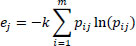
where:
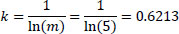
because each entropy value is calculated from 5 techno-economic parameters.
Entropy values
| Process Route | ej |
|---|---|
| CHPO CA | 0.9385 |
| CHPO | 0.9525 |
| POSM | 0.9103 |
| POTBA | 0.9665 |
| HPPO | 0.9705 |
| CuPO | 0.9358 |
Step 5: Compute divergence dj
Formula: dj = 1 ej
| Process route | dj |
|---|---|
| CHPO CA | 0.0615 |
| CHPO | 0.0475 |
| POSM | 0.0897 |
| POTBA | 0.0335 |
| HPPO | 0.0295 |
| CuPO | 0.0642 |
Total divergence:
0.0615 + 0.0475 + 0.0897 + 0.0335 + 0.0295 + 0.0642 = 0.3259
Step 6: Compute final entropy weights wj
Formula:

| Process Route | Weight (%) | |
|---|---|---|
| CHPO CA | 0.1887 | 18.87 |
| CHPO | 0.1458 | 14.58 |
| POSM | 0.2752 | 27.52 |
| POTBA | 0.1027 | 10.27 |
| HPPO | 0.0906 | 9.06 |
| CuPO | 0.1970 | 19.70 |
Appendix B. Detailed TOPSIS Calculation for Total Revenue
This appendix illustrates, step by step, how the Total Revenue row in the weighted normalized matrix was obtained and how it leads to the final TOPSIS closeness coefficient of 0.5280, which corresponds to Rank 1.
Appendix B1. Source values used for Total Revenue
The weighted normalized values for Total Revenue are obtained from the following two sources:
| Process Route | Weight, wj |
|---|---|
| CHPO CA | 0.1887 |
| CHPO | 0.1458 |
| POSM | 0.2752 |
| POTBA | 0.1027 |
| HPPO | 0.0906 |
| CuPO | 0.1970 |
| Parameter | CHPO CA | CHPO | POSM | POTBA | HPPO | CuPO |
|---|---|---|---|---|---|---|
| Total Revenue | 0.2913 | 0.1977 | 0.8390 | 0.6638 | 0.2737 | 0.2886 |
Appendix B2. Calculation of weighted normalized values for Total Revenue
The weighted normalized matrix is calculated using Equation:
vij = wj x rij
For the Total Revenue row, the vector-normalized values from Table 5 are multiplied by the corresponding entropy weights from Table 4.
CHPO CA
v21 = 0.2913 × 0.1887 = 0.05496831 ≈ 0.0550
CHPO
v22 = 0.1977 × 0.1458 = 0.02882466 ≈ 0.0288
POSM
v23 = 0.8390 × 0.2752 = 0.2308928 ≈ 0.2309
POTBA
v24 = 0.6638 × 0.1027 = 0.06817526 ≈ 0.0682
HPPO
v25 = 0.2737 × 0.0906 = 0.02480022 ≈ 0.0248
CuPO
v26 = 0.2886 × 0.1970 = 0.0568542 ≈ 0.0568
| Parameter | CHPO CA | CHPO | POSM | POTBA | HPPO | CuPO |
|---|---|---|---|---|---|---|
| Total Revenue | 0.0550 | 0.0288 | 0.2309 | 0.0682 | 0.0248 | 0.0568 |
This row matches the Total Revenue row reported in Table 6.
Appendix B3. Ideal best and ideal worst values used for TOPSIS
The weighted normalized row for Total Revenue is then compared with the positive ideal solution and the negative ideal solution.
| Process route | CHPO CA | CHPO | POSM | POTBA | HPPO | CuPO |
|---|---|---|---|---|---|---|
| Positive ideal solution, V+ | 0.1492 | 0.0796 | 0.2309 | 0.0682 | 0.0576 | 0.1566 |
| Negative ideal solution, V - | 0.0528 | 0.0288 | 0.0684 | 0.0269 | 0.0248 | 0.0557 |
Appendix B4. Calculation of separation from the positive ideal solution
The separation from the positive ideal solution is calculated using Equation:
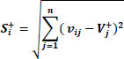
For Total Revenue:
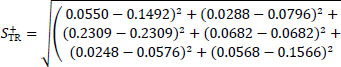
Now calculate each squared term:
(0.0550 - 0.1492)2 = (-0.0942)2 = 0.00887364
(0.0288 - 0.0796)2 = (-0.0508)2 = 0.00258064
(0.2309 - 0.2309)2 = 0
(0.0682 - 0.0682)2 = 0
(0.0248 - 0.0576)2 = (-0.0328)2 = 0.00107584
(0.0568 - 0.1566)2 = (-0.0998)2 = 0.00996004
Summing all terms:
0.00887364 + 0.00258064 + 0 + 0 + 0.00107584 + 0.00996004 = 0.02249016
Taking the square root:

Appendix B5. Calculation of separation from the negative ideal solution
The separation from the negative ideal solution is calculated using Equation:
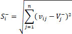
For Total Revenue:
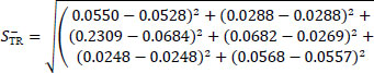
Now calculate each squared term:
(0.0550 - 0.0528)2 = (0.0022)2 = 0.00000484
(0.0288 - 0.0288)2 = 0
(0.2309 - 0.0684)2 = (0.1625)2 = 0.02640625
(0.0682 - 0.0269)2 = (0.0413)2 = 0.00170569
(0.0248 - 0.0248)2 = 0
(0.0568 - 0.0557)2 = (0.0011)2 = 0.00000121
Summing all terms:
0.00000484 + 0 + 0.02640625 + 0.00170569 + 0+0.00000121 = 0.02811799
Taking the square root:

Appendix B6. Calculation of the relative closeness coefficient
The relative closeness coefficient is calculated using Equation:

For Total Revenue:
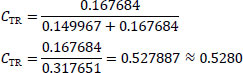
| Parameter | Si+ | Si- | Ci | Rank |
|---|---|---|---|---|
| Total Revenue | 0.1499 | 0.1677 | 0.5280 | 1 |
| Raw Material Cost | 0.1707 | 0.1440 | 0.4576 | 2 |
| Utilities Cost | 0.2050 | 0.0618 | 0.2316 | 3 |
| Investment Cost | 0.1978 | 0.0561 | 0.2209 | 4 |
| Fixed Cost | 0.2174 | 0.0512 | 0.1905 | 5 |